- Published on
Data Engineering Zoomcamp, Week 4: Analytics Engineering with dbt
As defined on their website, dbt™ is a SQL-first transformation workflow that lets teams quickly and collaboratively deploy analytics code following software engineering best practices like modularity, portability, CI/CD, and documentation.
In this week's post, I reflect on some of the initial challenges I faced while working through the Week 4 module, particulary regarding the datasets needed. I'll offer an interesting solution in which I admitedlly spent way too much time implementing, but enjoyed nonethless.
We'll start by touching on the prerequisites required for the Module, prior to diving into potential memory issues in Mage data pipelines and timestamp precision complexities that arise when converting parquet to a pandas dataframe. Lastly, I'll rehash the steps we performed in the module to successfully create a dbt model we can use for further analysis with Google's BI solution, Looker Studio.
I spent a lot of time putting this post together and I hope you find it insightful. If you have any questions or would simply like to connect, feel free to add me on LinkedIn!
Lastly, the contents of this post are based on my learnings from Week 4 of the DTC Data Engineering Zoomcamp, which you can find at this GitHub repository.
- Prerequisites
- Potential Issues
- Updated Mage Pipeline
- Creating and Deploying a dbt™ Model
- Data Visualization
- Conculsion
Prerequisites
Before we can get into this module, there are a handful of datasets we need. If you haven't done this already, DTC provides a quick hack to perform this which I believe should set you on the right path. Otherwise, I will go into some issues I had while ingesting the data with Mage below and provide an updated solution that I have personally tested on each dataset. If you have all this already setup, feel free to skip ahead.
- 2019 and 2020 Yellow NY Taxi data
- 2019 and 2020 Green NY Taxi data
- 2019 FHV Taxi data (homework)
Potential Issues
Insufficient Memory
I'll start by saying I was wrong in my Week 3 post. More specifically, I designed a Mage pipeline with the purpose of ingesting all of the necessary taxi data for our module (green, yellow & fhv). When I initially loaded all of the data into GCS, I used this local python script and only then did I explore implementing something similar with Mage. The issue is I only tested one taxi service (green) and one year (2019), which was successful, but I found a plethora of issues when attempting to ingest the yellow taxi data, etc with Mage after the fact. My pipeline was failing because I was loading too much data into memory, more than my Docker container was configured to handle. This would cause the pipeline to fail and ultimately I would have to restart the docker container as it would freeze up due to memory constraints, resulting in one big headache.
This lead me on a search for a solution to my memory problem, but this is not your grandpas memory problem. The first thing I discovered was what Mage calls dynamic blocks. Dynamic blocks allow you to split up blocks, such as a data loader, into multiple pieces and run them in parallel. For example, we can take our data loader and rather concatenating all of our taxi data into one dataframe, we can split it into separate blocks that can each be loaded into memory in parallel or even sequentially.
At first, I ran 4 blocks in parallel (4 data loader blocks), each block represented a parquet file containing taxi data for a specific month (i.e. Jan, Feb, March). At this point I assumed I had cracked the code, but still found my pipleine was failing due to insufficient memmory, once again.
The solution I arrived at was to configure my Data Loader as a dynamic block and to then modify the concurrency of said blocks within the metadata.yml file belonging to my pipeline to a value of 1. This enabled my pipeline to run each dynamic block sequentially (1 by 1) until each file was loaded, rather than appending all the files to a single dataframe.
My understanding is that only 1 dynamic child block will run at a time, which will help alleviate potential memory constraints, but will be effectively much slower. Alas, I am beholden to the specifications of my personal computer, in which I've allocated 8 GBs of memory to docker as well as 4 vCPUs. Were I to configure this mage pipeline to run on a remote container, provisioned with greater memory and compute, I could likely increase the concurrency figure as necessary, effectively speeding up my pipeline runtime.
concurrency_config:
  block_run_limit: 1
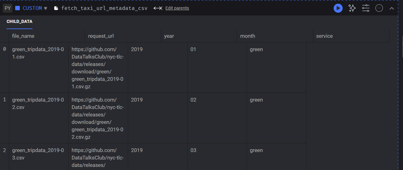
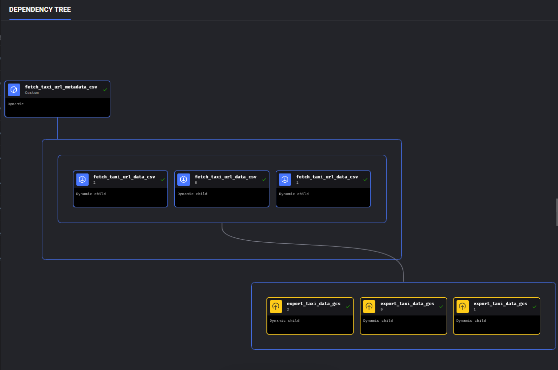
At the end of this section, I've provided an example snapshot of what a Mage pipeline with dynamic blocks looks like during execution. For the sake of simplicity, I only loaded 3 months of Taxi data. The pipeline works as follows, the fetch_taxi_url_metadata_csv block is configured as a "dynamic block". It iterates through a range of 12, representing the total months in a year, then appends the url data for each file to a list of dictionaries that is referenced in our return statement as [download_info] to be passed unto our child block fetch_taxi_url_data_csv. The output of this block would look like the following image:
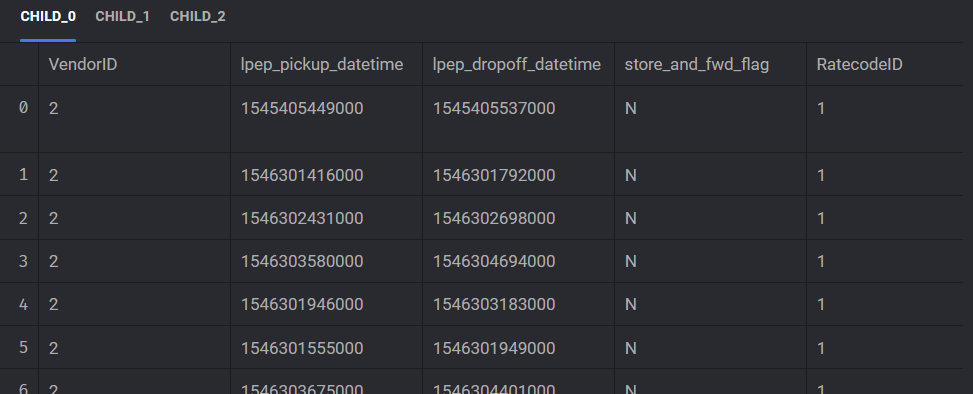
Next we have a "dynamic child" block. This secondary data loader takes the url for each item in our download_info list and retrieves the csv data for each month, i.e. January, February and March and returns each as a separate dataframe labeled "child_0, child_1 and child_2". Lastly, our data exporter exporter_taxi_data_gcs takes each child block and exports the dataframe into google cloud storage.
This parallelization allows us flexibility in a handful of ways. We can speed up our pipeline by increase the amount of concurrenct blocks we want to run. If we set this figure to 3, all 3 of our data loaders will run in parallel, instead of sequentially. If we set the concurrency value to 1, only one child block will run at a time, effectively reducing the amount of data we are loading into memory at one time. You can contrast this with some of the Mage pipelines we built in the earlier modules, where we loaded all of the csv data into one singular dataframe value. This may work in a pinch, but does not scale well the more data we load in. Particularly the yellow taxi data, which contains the most amount of records was giving me this issue!
Timestamp Precision
I want to first note that this issue can be avoided simply by using the csv data in the DTC repo, but I was curious of the parquet format and wanted to explore that further by going directly to the source. In hindsight, the following issue was avoidable but regardless I want to share my findings as similar issues are likely to appear if you work in data engineering.
In my work with FHV taxi trip data, I encountered a notable issue while loading the data. My Mage pipleline was breaking due to the following error:
pyarrow.lib.ArrowInvalid: Casting from timestamp[us] to timestamp[ns] would result in out of bounds timestamp: 33106123800000000
This error arises from a common situation in data handling.
Our Parquet files store timestamps in microseconds. When converting these to nanoseconds, the standard practice in Pandas, each value is multiplied by 1000 (since 1 microsecond = 1000 nanoseconds). However, this operation can push the value beyond the maximum limit of a 64-bit signed integer, used by both Pandas (datetime64[ns]) and Parquet for timestamp storage. This limit is or . Exceeding this threshold results in an 'out of bounds' error.
For instance, our original value of 33,106,123,800,000,000 (in microseconds) becomes 33,106,123,800,000,000,000 when converted to nanoseconds, a figure represented as 3.31061238e+22. This value significantly surpasses the 64-bit limit of 9,223,372,036,854,775,807. In practical terms, the maximum year that can be represented in nanoseconds is approximately Fri Apr 11 2262 23:47:16. Our value, corresponding to February 3, 3019, at 17:30, clearly exceeds this boundary.
To illustrate these out-of-range values, refer to the following table. As a Data Engineer, encountering such erroneous timestamps necessitates a decision on handling. In our bootcamp, I chose to convert out-of-bound timestamps to Pandas' NaT (not-a-time) type, essentially treating them as null values. In real-world scenarios, alternative approaches might be considered.
| Datetime | Microsecond Timestamp | Nanosecond Equivalent (Microsecond * 1000) | Within 64-bit Range? |
|---|---|---|---|
| 1970-01-01 00:00:01 | 1,000,000 | 1,000,000,000 (1e9) | Yes |
| 2262-04-11 23:47:16 | 9,223,372,036,854 | 9,223,372,036,854,000 (9.22e15) | Yes |
| 2262-04-11 23:47:16.854775 | 9,223,372,036,854,775 | 9,223,372,036,854,775,000 (9.22e18) | Yes |
| Out of Bounds | 9,223,372,036,854,776 | 9,223,372,036,854,776,000 (9.22e18) | No |
| Out of Bounds | 10,000,000,000,000,000 | 10,000,000,000,000,000,000 (1e19) | No |
| Out of Bounds | 33,106,123,800,000,000 | 33,106,123,800,000,000,000 (3.31e19) | No |
Updated Mage Pipeline
If your curious about my implementation of Mage, you can take a look at my repo which contains the pipeline I outlined above, which is specifically named ingest_all_taxi_data_gcs_csv.
Creating and Deploying a dbt™ Model
dbt™ stands as a bridge between data engineering and software engineering, introducing practices from the latter to enhance the management and deployment of SQL code. Just as Python benefits from a wealth of libraries, dbt offers a suite of packages equipped with pre-written macros. These macros, akin to Python functions, simplify and streamline the creation and maintenance of our data models, making the overall process more efficient and manageable.
Setup
Setting up a dbt project involves several key steps that lay the foundation for efficient data modeling and transformation. Let's walk through the process of creating a new dbt project.
Create a project
If you haven't already, you can signup for an account here
Once signed in, you will need to create a DBT Account, which may sound confusing considering we just setup an account, but think of it as a directory that holds all of your dbt projects. I named mine DTC DE Zoomcamp.
If you are having trouble, refer to the documentation provided by DTC in the Week 4 readme for setuping dbt cloud.
Connect project to Github Repository
Before we create and deploy our dbt project, we will need to link dbt to our github repository, more specifically a cloned repository containg the Week 4 "04-analytics-engineering" folder. After we link the repository,
Note: I recommend using the GitHub connector instead of the Git Clone option, as I later had issues with deploying a CI Job due to using the latter.
Next you will need to set the project subdirectory to the location of of our dbt project, which is within the taxi_rides_ny folder. 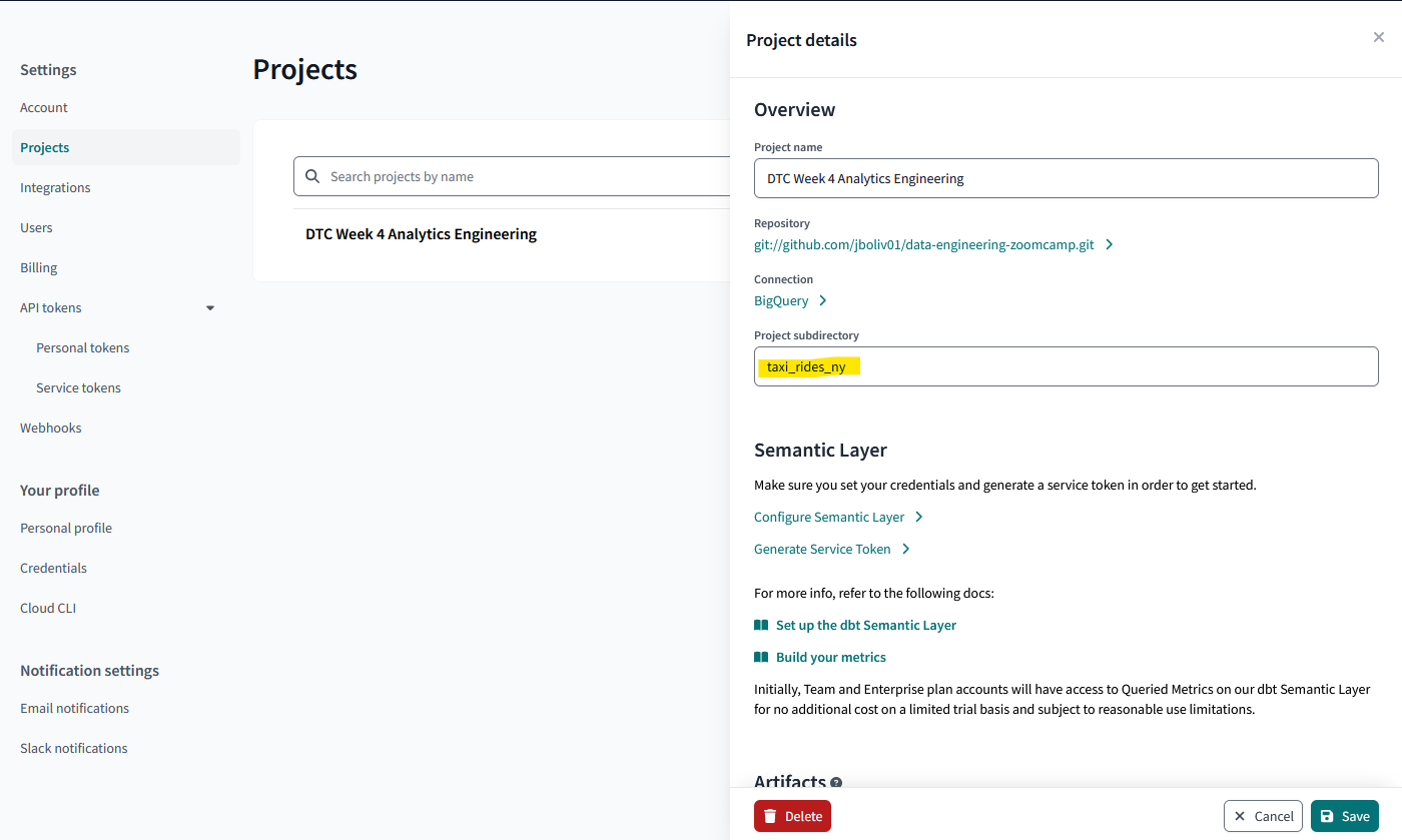
Connect project to Data Warehouse
Lastly, we need to link our project to our BigQuery Data Warehouse. This is pretty straight forward, as it allows us to import the service account key we generated in the previous module. At this point, you likely already have one downloaded, but see my previous post here if you need a refresher.
Define dbt Models
Staging Models
Now that our project has been configured with the necessary settings, it's time to open up the dbt IDE and get started. Once the IDE has loaded, one of the first things you may notice is a button prompting us to "Create Branch". It is best practice to create feature branches, which are any changes we want to make to our original code, prior to submitting whats known as a "pull request" that generally has to be reviewed by others to assure there are no breaking changes. Once reviewed, the pull request can then be merged into our main branch. In this case, we own the repository so we have the ability to create a feature branch, update our code, submit a pull request and approve it.
Under our dbt project taxi_rides_ny, there should be a models folder containing two subfolders: staging and core. The staging model will define the schema of our taxi data as well as some test suites. The core model will contain our fact table, which will ultimately join our green and yellow taxi data together as one table for further analysis.
Under staging, we defined the schema of our tables in schema.yml. Dbt then allows us to auto-generate the models for our staging tables, green_tripdata and yellow_tripdata, by clicking "Generate model".
sources:
  - name: staging
    database: dtc-de-zoomcamp-12345
     # For postgres:
      #database: production
    schema: ny_taxi

    tables:
      - name: external_green_tripdata
      - name: external_yellow_tripdata
      - name: external_fhv_tripdata
         # freshness:
           # error_after: {count: 6, period: hour}
For the sake of this blog post, I will share the external_fhv_tripdata.sql model I first auto-generated but then later modified to be consistent with the green and yellow tripdata models.
{{ config(materialized="view") }}

with
    fhv_tripdata as (
        select *, row_number() over (partition by pulocationid, pickup_datetime) as rn
        from {{ source("staging", "external_fhv_tripdata") }}
    )

select
    {{ dbt_utils.generate_surrogate_key(["pulocationid", "pickup_datetime"]) }}
    as tripid,
    {{ dbt.safe_cast("dispatching_base_num", api.Column.translate_type("integer")) }}
    as dispatching_base_num,
    cast(pickup_datetime as timestamp) as pickup_datetime,
    cast(dropoff_datetime as timestamp) as dropoff_datetime,
    {{ dbt.safe_cast("pulocationid", api.Column.translate_type("integer")) }}
    as pickup_locationid,
    {{ dbt.safe_cast("dolocationid", api.Column.translate_type("integer")) }}
    as dropoff_locationid,
    sr_flag,
    affiliated_base_number

from fhv_tripdata
--where rn = 1

-- dbt build --select <model.sql> --vars '{'is_test_run: false}'
{% if var("is_test_run", default=true) %} limit 100 {% endif %}
Compiling the model will allow us to see the output of the macros we are using.
with
    fhv_tripdata as (
        select *, row_number() over (partition by pulocationid, pickup_datetime) as rn
        from `dtc-de-zoomcamp-12345`.`ny_taxi`.`external_fhv_tripdata`
    )

select
    to_hex(md5(cast(coalesce(cast(pulocationid as string), '_dbt_utils_surrogate_key_null_') || '-' || coalesce(cast(pickup_datetime as string), '_dbt_utils_surrogate_key_null_') as string))) as tripid,
    safe_cast(dispatching_base_num as INT64) as dispatching_base_num,
    cast(pickup_datetime as timestamp) as pickup_datetime,
    cast(dropoff_datetime as timestamp) as dropoff_datetime,
    safe_cast(pulocationid as INT64) as pickup_locationid,
    safe_cast(dolocationid as INT64) as dropoff_locationid,
    sr_flag,
    affiliated_base_number

from fhv_tripdata
--where rn = 1

-- dbt build --select <model.sql> --vars '{'is_test_run: false}'
 limit 100
Running the following dbt command will create the staging table in google bigquery based on the model we have specified.
dbt build --select +stg_external_fhv_tripdata+ --vars '{'is_test_run': 'false'}'
Core Models
Within the Models folder, we should have two subfolders, Core and Staging. With our staging model defined, we now need to create a our finalized Fact model. This is where we will perform any necessary joins to our table. We no longer need to worry about the data types in our schema as we have handled that in our staging table model. In the case of our fact_fhv_trips.sql model, we are selecting the necessary columns we want in our finalized model and performing two inner-joins to our dim_zones model, which has a where clause to filter out any zones with a borough type of unknown. This was a requirement for one of the homework questions in the week 4 module.
{{
    config(
        materialized='table'
    )
}}

with external_fhv_tripdata as (
    select *,
    'FHV' as service_type
    from {{ ref('stg_external_fhv_tripdata') }}
),
dim_zones as (
    select * from {{ ref('dim_zones') }}
    where borough != 'Unknown'
)

SELECT
external_fhv_tripdata.dispatching_base_num,
external_fhv_tripdata.affiliated_base_number,
external_fhv_tripdata.pickup_locationid,
external_fhv_tripdata.dropoff_locationid,
external_fhv_tripdata.pickup_datetime,
external_fhv_tripdata.dropoff_datetime,
external_fhv_tripdata.service_type
FROM external_fhv_tripdata
inner join dim_zones as pickup_zone
on external_fhv_tripdata.pickup_locationid = pickup_zone.locationid
inner join dim_zones as dropoff_zone
on external_fhv_tripdata.dropoff_locationid = dropoff_zone.locationid
Once finished, the lineage of our dbt model should look something like this:
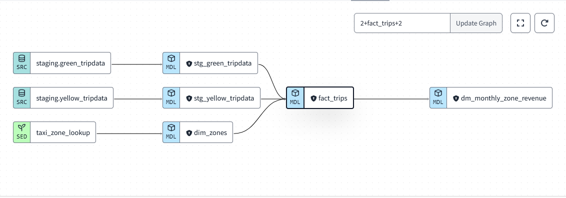
Model Schema
In our schema.yml file we can
sources:
  - name: staging
    database: dtc-de-zoomcamp-12345
    schema: ny_taxi

    tables:
      - name: external_green_tripdata
      - name: external_yellow_tripdata
      - name: external_fhv_tripdata
and within a downstream model, we can use:
select * from {{ source('staging', 'external_fhv_tripdata') }}
Which will be compiled to:
select * from dtc-de-zoomcamp-12345.ny_taxi.external_fhv_tripdata
We can also define tests we would like to execute against our models on build time. i.e. we want to test our tripid column to ensure each field is unique and not a null value, in the instance below, a warning will be thrown if a record does not meet that criteria. A warning will not stop our model from deploying, but if we were to change the severity type to error, this would stop our deployment. This can all be defined within our schema.yml file in the Staging subdirectory we've created within Models.
models:
  - name: stg_external_green_tripdata
    description: ""
    columns:
      - name: tripid
        data_type: string
        description: ""
        tests:
          - unique:
              severity: warn
          - not_null:
              severity: warn
Packages and Macros
dbt packages can be added in the packages.yml file, similar to how we added python dependencies for our docker container in the requirements.txt file in module 1. We utilized some of these macros while building out our staging models.
db_utils package provides us with macros we can (re)use across dbt projects, such as the generate hash key macro we used in our staging model to create a unique primary key.
The dbt-labs/codegen package contains a handful of useful macros that make writing a model more efficient. For example, we can use the generate_model_yaml macro to generate the YAML for a list of models we can then paste into our schema.yml file. This saves us time when defining the schema of our tables.
{% set models_to_generate = codegen.get_models(directory='marts', prefix='fct_') %}
{{ codegen.generate_model_yaml(
    model_names = models_to_generate
) }}
Project Variables
Variables can be defined within the dbt_project.yml to provide data to models for compilation. i.e. the payment_type_values variable is a field that is present in both green and yellow taxi data.
Defined as follows in dbt_project.yml:
vars:
  payment_type_values: [1, 2, 3, 4, 5]
and later accessed in the schema.yml for our project under both the green and yellow taxi models using the the {{ var('...') }} function:
 - name: payment_type
        data_type: int64
        description: ""
        tests:
          - accepted_values:
              values: " {{ var('payment_type_values') }}"
Deployment Jobs (CI/CD)
dbt makes creating a CI job fairly simple. We will start by creating a new environment within dbt under Deploy -> Environments.
When configuring the deployment job, we'll enable generate docs on run and run source freshness.
A Continious Integration job will ensure when any new changes are successfully merged into main, a job will automatically be deployed and any updates will be applied to our production model.
dbt effectively describes how CI works in their documentation: "When you set up CI jobs, dbt Cloud listens for webhooks from your Git provider indicating that a new PR has been opened or updated with new commits. When dbt Cloud receives one of these webhooks, it enqueues a new run of the CI job.
dbt Cloud builds and tests the models affected by the code change in a temporary schema, unique to the PR. This process ensures that the code builds without error and that it matches the expectations as defined by the project's dbt tests...
When the CI run completes, you can view the run status directly from within the pull request. dbt Cloud updates the pull request in GitHub, GitLab, or Azure DevOps with a status message indicating the results of the run. The status message states whether the models and tests ran successfully or not.
dbt Cloud deletes the temporary schema from your data warehouse when you close or merge the pull request."
We can also setup a Deploy job simply to run our model at a scheduled cadence to ensure any new data that may have been ingested into our data source will be captured in our production models.
Data Visualization
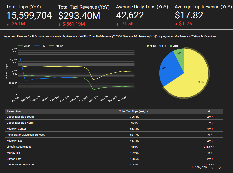
Now that we have solidified our data model, we can use Google's data looker studio to create a dashboard for analysis. Naturally, Google's BigQuery is already built in as a data connector, which makes accessing our data a straightforward process. I used our newly created fact_trips model to build a simple dashboard which aims to convey how Taxi Trips and Revenue were effected by covid from 2019-2020.
Conculsion
For more insights or to discuss these topics further, feel free to connect with me on LinkedIn. I'm really excited to dive into the coming modules as the zoomcamp is coming to a close in the coming months.